Introduction
A common problem in the medical imaging community is the alignment of similar MRI scans for comparison. Patients may, for example, move their head during a brain MRI, corresponding to transformations in 2D output scans before and after the patient’s movement. This problem is better known as the image registration problem, and its solution is a critical step in examination of medical images.
Another class of problems encountered in the larger computer vision community is the segmentation problem. Image segmentation is the task of attributing certain neighborhoods of pixels in an image to an associated class. As one can imagine, this has a wide range of useful applications.
In this project, a method for middle-coronal registration and segmentation was realized using 6 training and 2 validation samples, each of which had a manually segmented and non-segmented version that labeled four portions of the brain: Left Cerebral Cortex, Right Cerebral Cortex, Left White Matter, and Right White Matter. The general structure of the imaging pipeline was as follows:
- Image preprocessing
- Registering training (moving) images to validation (fixed)
- Image transformation
- Interpolation
- Optimization on defined objective
- Applying optimal transformation parameters to corresponding segmentations
- Label fusion strategy
- Similarity metric (e.g. Jaccard) between automatic and manual segmentation
The intuition for this pipeline is as follows: we have a total of 8 training/validation samples with labeled segmentations provided by human experts (the “manual” segmentations). We want to take a given test subject’s MRI scan, perform transformations such that the images are aligned as closely as possible, and then use the segmentations we have from human experts of the training images to automatically produce a segmentation of the new test scan (“automatic”). Of course, during training, we do not have access to test subjects, so we use 2 of the 8 training samples as validation subjects.
Inside of this setup several parts were tunable and modifiable to achieve a better resultant automatic segmentation, and the goal was to find a setup that resulted in a relatively high Jaccard overlap between the automatic segmentation and the manual one. Throughout this process, visualization of the processing, registration, and segmentation procedures was crucial to determining the effectiveness of each procedure.
Image preprocessing
The first significant improvement to the pipeline was max-intensity normalizing each image before inputting it into any optimization method. This greatly accelerated the optimization procedure runtime and in running the program yielded outputs with a lower sum-of-squared differences (SSD) objective. It seemed that the derivative-free optimization methods used were better equipped for floating point arithmetic in the range [0,1] provided by max-intensity normalization.
Another candidate preprocessing technique was a Gaussian smoothing of the fixed and moving images. The motivation for this was that individual scans of the brain, however well aligned, will exhibit some innate differences. By applying a Gaussian smoothing kernel with sufficiently low variance σ, each image loses some very high frequency components that are unimportant in the segmentation problem, and thus can be disregarded. Ideally, this provides a more robust registration/segmentation pipeline that’s less sensitive to discrepancies between training images and testing images, thereby preventing the segmentation outputs from being overfitted to the training images. On the other hand, a large σ for the Gaussian kernel is undesirable as the registration becomes meaningless if the boundary regions for the regions of interest (or the scan itself) are indistinguishable, so a smaller σ (corresponding to the 3x3 or 5x5 kernel) is more suitable.
The next preprocessing technique considered was histogram equalization of intensities. For this task , two popular histogram equalization techniques were considered: the exact histogram equalization (EHE) algorithm covered in class and the contrast-limited adaptive histogram equalization (CLAHE) algorithm. For the image registration task in MRI-scans, CLAHE is preferred over EHE because EHE produces unnecessarily high contrasts and transforms intensity relative to global statistics. The registration SSD error for all images using CLAHE as opposed to EHE was significantly smaller. Interestingly, EHE made the registration error worse than that without any histogram equalization by approximately 10-20% per image, while CLAHE improved upon it by about 15%, so CLAHE was kept. Note that these approximate improvements are dependent on other image preprocessing decisions. The chosen parameters for the CLAHE procedure were 8x8 tile size with a clip limit of 2.0, which are the default of the OpenCV package. This meant that in the resulting histogram, the a pixel neighborhood consisted of the 8x8 region in which it was centered and that the top of the histogram was plateaued at an intensity equal to twice the minimum intensity of the neighborhood, with the histogram redistributed when an intensity pushes the peak over the clip limit.
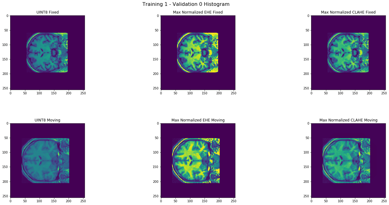
Histogram transforms of MRI Scans
Image registration
In the registration problem, a moving image and a fixed image should be aligned as closely as possible. The objective function used to determine how close two images are was the sum-of-squared differences (SSD), with an added regularization term γ to encourage small transformation parameters, though this did not have a significant effect on registration results. At first, a geometric transformation (rotation, scale, 2-D shift) was considered. Later, a 2-D scaling was enabled and the general class of affine transformations was considered. In most cases, the provided training/validation images were similarly scaled to begin with so scale parameters were between 0.9 and 1.1 in both directions, and significant translations (>10 pixels) were not observed.
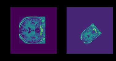
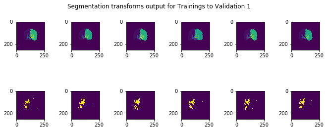
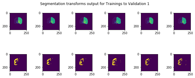
Sample Image Transformation
For the optimization routine used in the registration, a derivative-free algorithm was deemed desirable in place of a derivative-based method like gradient descent. The Nelder-Mead simplex method was the first candidate algorithm, but this method was slower than the Powell conjugate direction method adopted later. To ensure better optimization results, 1,000 iterations were allowed (though no registration took 1,000 iterations) and the convergence criterion parameter was decreased from the default of 1e-4 to 1e-7.
Label fusion strategies
The naïve mode-based label fusion strategy consisted of taking a mode of the segmentation for a pixel along all training images to decide the labels of the test segmentation.
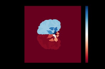
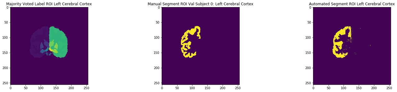
Majority voted label fusion technique
The natural next step was to reduce uncertainty by having labels in the majority vote with discrepancy removed. After taking the mode of the segmentations produced by the training images, the pixels with disagreement over some “bound” parameter were removed. This occurred most often near the boundaries of ROIs, as can be seen in the image below:
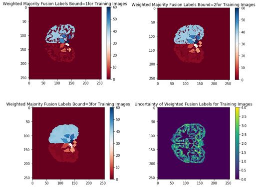
Modified label fusion technique
The intuition behind this modified voting process was that the “agreed upon” regions of overlap would prevent false negatives from occurring in the segmentation near boundary regions. However, this proved not to significantly alter the validation or test results, generating slight improvement if any.
One last strategy for maintaining contiguous predicted segmentations was attempting to remove disconnected pixels from consideration. For example, in the final binary mask of the ROI, a small number pixels far from the actual ROI were active, presumably as a byproduct of ambiguity in validation label votes or a processing step. Pixels with fewer than a threshold number of active neighbors were turned off, using a sum filter convolved on the binary segmentation result that decided which pixels had enough active neighbors to remain in the image.
Conclusions and Future Work
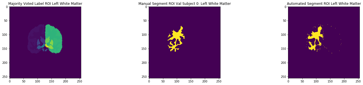
The test subjects given were registered with respect to the training and validation images, and compared with the manual test segmentations held by the course instructors. Upon submission of several different results to the class Kaggle competition, it seemed that the Dice score was nearly 0.66, corresponding to a test Jaccard overlap of around 0.49 on average for the test results, a 0.14 improvement on the competition baseline of 0.35. A sample of the results can be seen below:
There are several areas I would research and implement further given more time to explore. First, there are a litany of hyperparameters to tune in each step of the process, and more complex methods introduce even more hyperparameters, so either manually tuning these or using automatic means such as Bayesian optimization over the hyperparameter space would be an interesting point of enquiry. Additionally, even though I attempted to improve the voted label fusion technique, both methods were somewhat crude and another point of research would be to find a more elegant solution to that: for example, it could be that one training image is contributing to more noise, for example, and a weighted scheme would ideally take that into account. Next, with regards to the segmentation problem, it is possible that machine-learning methods in computer vision such as convolutional neural networks (CNN) could find a mapping between the space of pixel intensities by pixel position to the space of pixel segmentation labels, providing an end-to-end solution that, due to spatial invariance introduced in these methods, may bypass the registration problem altogether. Given only 6 training examples, machine learning methods may be prone to overfitting themselves, but exploring this area with deep learning or traditional ML methods may provide more insights.