Now that summer is almost over, it’s time for me to recap my experience in a summary. I’ve linked a lot of the resources I’ve used on this post.
After finals in May I took the Udacity Deep Learning Course from Google. With the help of Ian Goodfellow’s textbook Deep Learning, I built a foundation about basic neural network frameworks, such as convolutional and recurrent neural nets. I highly recommend these resources with Andrew Ng’s Machine Learning class on Coursera and Stanford’s Computer Vision course for anybody looking for an introduction to deep learning, as they’re extremely popular and thorough. I also learned how to use Tensorflow and wrappers like tflearn to implement machine learning models.
Beginning in June, I worked on a deep learning project that incorporated supervised learning as well as reinforcement learning with my friend and colleague from the Organic Robotics Lab, Chris Larson. The premise of my research was similar to the AlphaGo experiment, except with checkers. The main objective was to see if a machine learning model trained similarly to the AlphaGo one would beat the superhuman checkers players that exist today. Another point of interest was the fact that checkers is a solved game. What this means is that it can be proved that each move a perfect player makes is, in fact, the optimal move. We thought that this may be an interesting point of inquiry, to see how much training is required to be “perfect”.
We tried to mimic checkers boards (essentially, possible state representations) using a generative adversarial network. First, I’ll explain what a generative adversarial model is. This is a deep learning paradigm which Ian Goodfellow invented paper. Since the introduction of the original model, people have come up with a litany of variants. In any case, a vanilla generative adversarial model actually consists of two neural networks: a generator and a discriminator. Say you have a set of images (though your dataset can really be anything). The job of the generator is to take random noise as input and output an image that replicates something from your set of images. Meanwhile, the discriminator’s job is to decide whether an image you feed into it is a “real” image from your dataset or a “fake” one from the generator. As you train the models, the networks play what’s called a minimax game (inspired from game theory), and eventually you want the discriminator to be unable to differentiate between the generator output and real images. All adversarial frameworks are based on this idea.
My purpose for using GANs was to try to replicate checkers boards, effectively augmenting our training data. The idea was that the generator would be able to learn the legitimacy of checkers-boards spaces so that valid boards were created, which would not be possible if random Gaussian noise was added to training samples. Eventually, it turned out we had sufficient data and didn’t need a GAN, but the GAN models I built taught me some really cool tricks:
batch norm- batch normalization is a way to reduce internal covariate shift in your data. Essentially, batch norm is trying to make sure the relationships between the variables in your data don’t change between batches of data, so that high-order gradient updates do not increase loss. This is explained in detail on this excellent post.
sparsity- the problem with our checkers encoding was that we were asking the generator to replicate a 8x4 array representing a board with mostly 0s and a couple 1s,-1s,3s,and-3s (representing self/opponent pieces and normal pieces and kings respectively). Therefore, it was really easy for the generator to spit out game boards that’d be near-endgame scenarios with few filled pieces and mostly empty positions on the board. This wasn’t wrong, per se, but it gave an interesting insight into how GANs work. If this were to be attempted again, there would certainly need to be some preventative conditioning in place (perhaps by adding parameters to the loss function discouraging sparse boards).
ReLUs and leaky ReLUs- In normal linear rectified units (ReLUs), the output is y=x if x>0 and y=0 if x<0. The problem is that when a neural network performs gradient updates, if x<0, the gradient will be 0 (because dy/dx of y=0 is 0), leading to a “dying ReLU”. A leaky ReLU changes this by making y=αx for x<- where α is some small number, like 0.01.
Reinforcement learning was one of the coolest things I learned about over summer. One great resource for all of this information is Dave Silver’s Reinforcement Learning course and its associated YouTube lectures. Another useful resource is this post from Tambet Matiisen.
The idea behind reinforcement learning is very human: you learn from rewards. If you do something right, you “win”, or get a positive reward signal. Conversely, if you “lose”, there’s a negative reward signal. As you practice a task repeatedly, you get better at it, and positive rewards become likelier.
Now we can formalize this a little further. Consider an agent that is being trained through reinforcement learning. At first, let’s say it takes actions randomly. The action it takes has some consequence, that we say is the new “state” of the agent. It’s easy to think about like a board game: the agent moves to a new position on the board, which affects its likelihood of winning the game (win/lose), and the new board position gives the player different options about how to proceed in the game. The “environment” determines this new state and associated reward, which the agent uses to make its next decision.
From AWS
What I just explained (still sort of informally) is called a Markov Decision Process (MDP). MDPs are fundamental to modeling decision-making, because it’s a simple definition with profound implications. Formally, an MDP has:
- a finite set of states
- a set of actions that may or may not be dependent on the current state
- a set of rewards associated with an action taken
- a probability that an action in one state will lead the agent to another state
- a discount factor in [0,1] that essentially defines whether immediate rewards or potential future rewards take priority in decision-making
- Discount factor closer to 0 means priority is given to immediate rewards
- Discount factor closer to 1 means priority is given to future rewards
Then, if we sample a sequence of states, the “return” of that sequence can be expressed as the sum of the product of reward at each step and an exponent of the discount factor, which is an equation known as the Bellman Equation. This may sort of confusing to explain in words, so referencing Lecture 2 of Dave Silver’s course is recommended.
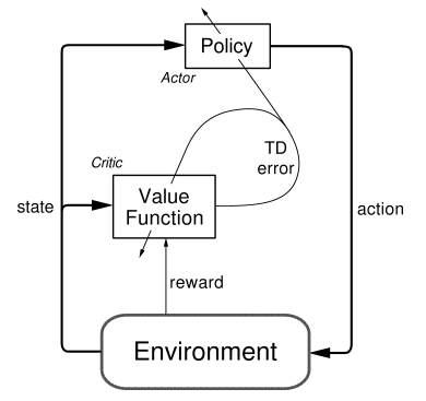
DDPG Model, from Patrick Emami
For my project, there were 2 well-researched algorithms that have recently been used for gameplay: Deep Q-learning and Deep Deterministic Policy Gradients (DDPGs). Both are reinforcement learning algorithms that are modeled as MDPs. At its core, Q-learning (not deep yet) is somewhat of a brute force approach: each possibility is randomly sampled, and once all possible rewards and states are observed, there is a recorded matrix of rewards corresponding to states. Basically, once you have this information, it is possible to simply refer to a matrix to determine which action yields the highest reward for a given state. In Deep Q-learning, the neural network essentially tries to iteratively fill in the values for the aforementioned matrix using the Bellman Equation. This may be effective in many cases, but with a game like checkers, this is rather inefficient computationally. To model expected reward, Therefore, we went with the second choice: DDPGs. DDPG’s are a form of “actor-critic” reinforcement learning, where there are two neural networks: one “actor” that is, in this case, the policy, and a “critic” that determines whether the policy’s chosen action was good. The policy is therefore simply some function that determines the action to be taken. To further the human analogy, it’s your “policy” to yield to pedestrians while driving or to bring an umbrella if it’s raining. For checkers, it’s easy to decide whether a game was won or lost with one neural network and then use that to update a policy. Specifically, the critic network can be trained as a traditional supervised-learning model would, with input games and output labels of whether the games were won or lost. Part of the ingenuity in AlphaGo that we took inspiration from comes from the next step: we use the supervised-learning policy that predicted good players’ moves and used that as the initial policy, similar to imitation learning. Now, we are further training an agent that is already trained at producing good moves from observation of human players. So, the cost function changes definition from similarity to good professional players’ moves to the likelihood of winning (i.e. expected reward). In other words, we shift from trying to maximize our moves to be like good pros’ to trying to maximize the chance of winning, based on playing many many games..
There’s two questions one may have: does starting with a supervised-trained policy actually improve the agent- would reinforcement learning beginning with an arbitrary policy not eventually achieve the same skill if it played as many games? Also, who does the model play to try to improve? The first question is difficult to answer: convergence is not always guaranteed and indeed depends on initial weights/biases (i.e. initial policy). In general, supervised training observing human professionals is probably a quicker way to get to a “world-class” level of checkers playing than is playing millions of games with an initially untrained model. In 2017, DeepMind updated the original AlphaGo result with AlphaGo Zero, which does not depend on the initial supervised-training procedure. The second question is easy to answer: it plays itself. To know if it’s improving over many games, anomalies that lead to victory (or “lucky” moves that aren’t actually always the best move in a given state) will be erased in favor of the true best move. To ensure that the policy isn’t optimized just for the deterministic model already trained, the most recently-trained policy plays against a random previous iteration of the policy (i.e. previous weights) that is saved to a ‘experience replay’ cache memory. This is sort of like randomly playing against an array of really good players at each step, learning from wins/losses, and then over many games learning the best way to beat all of them, and therefore maximize the likelihood of winning generally.
Though the mechanism is quite different, the processes of learning in reinforcement learning is similar to that of humans. During the summer, implementing this in Tensorflow was quite the challenge, but we eventually got a model that learned using DDPG.
In future research, the goal would be to parallelize this framework and enable it to train on cloud-deployed resource instances or, ideally, in-house computing resources. The memory and processing power needed to train the checkers framework fully is not feasible on my CPU-powered laptop, so it’s impossible to train the bot to any superhuman-level. We verified learning was taking place by observing gameplay, but it was difficult to say to what extent it was successful. Furthermore, while we created a Monte-Carlo Tree Search component that resembled AlphaGo’s, MCTS is only valuable once large-scale training takes place.